Chapter 4: Bare-Metal Switches

This chapter describes the bare-metal switches that provide the underlying hardware foundation for SDN. Our goal is not to give a detailed hardware schematic, but rather, to sketch enough of the design to appreciate the software stack that runs on top of it. Note that this stack is still evolving, with different implementation approaches taken over time and by different vendors. Hence, this chapter discusses both P4 as a language-based approach to programming the switch’s data plane, and OpenFlow as the first-generation alternative. We will introduce these two approaches in reverse-chronological order, starting with the more general, programmable case of P4.

4.1 Switch-Level Schematic

We start by considering a bare-metal switch as a whole, where the best analogy is to imagine a PC built from a collection of commodity, off-the-shelf components. In fact, a full architectural specification for switches that take advantage of such components is available on-line at the Open Compute Project (OCP). This is the hardware equivalent of open source software, and makes it possible for anyone to build a high-performance switch, analogous to a home-built PC. But just as the PC ecosystem includes commodity server vendors like Dell and HP, you can buy a pre-built (OCP-compliant) switch from bare-metal switch vendors such as EdgeCore, Delta and others.

Figure 18 gives a high-level schematic of a bare-metal switch. The Network Processing Unit (NPU)—a merchant silicon switching chip—is optimized to parse packet headers and make forwarding decisions. NPUs are able to process and forward packets at rates measured in Terabits-per-second (Tbps), easily fast enough to keep up with 32x100-Gbps ports, or the 48x40-Gbps ports shown in the figure. As of this writing, the state-of-the-art for these chips is 25.6 Tbps with 400-Gbps ports.

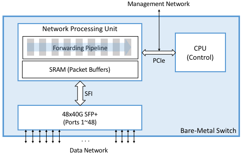
Figure 18. High-Level schematic of a bare-metal switch.

Note that our use of the term NPU might be considered a bit non-standard. Historically, NPU was the name given to more narrowly-defined network processing chips used, for example, to implement intelligent firewalls or deep packet inspection. They were not as general-purpose as the NPUs we are discussing in this chapter, nor were they as high-performance. The long-term trend, however, has been toward NPUs that match the performance of fixed-function ASICs while providing a much higher degree of flexibility. It seems likely that the current merchant silicon switching chips will make the earlier generation of purpose-built network processors obsolete. The NPU nomenclature used here is consistent with the industry-wide trend to build programmable domain-specific processors, including GPUs (Graphic Processing Units) for graphics and TPUs (Tensor Processing Units) for AI.

Figure 18 shows the NPU as a combination of SRAM-based memory that buffers packets while they are being processed, and an ASIC-based forwarding pipeline that implements a series of (Match, Action) pairs. We describe the forwarding pipeline in more detail in the next section. The switch also includes a general-purpose processor, typically an x86 chip, that controls the NPU. This is where BGP or OSPF would run if the switch is configured to support an on-switch control plane, but for our purposes, it’s where the Switch OS runs, exporting an API that allows an off-switch, Network OS to control the data plane. This control processor communicates with the NPU, and is connected to an external management network, over a standard PCIe bus.

Figure 18 also shows other commodity components that make this all practical. In particular, it is possible to buy pluggable transceiver modules that take care of all the media access details—be it 40-Gigabit Ethernet, 10-Gigabit PON, or SONET—as well as the optics. These transceivers all conform to standardized form factors, such as SFP+, that can in turn be connected to other components over a standardized bus (e.g., SFI). Again, the key takeaway is that the networking industry is now entering into the same commoditized world that the computing industry has enjoyed for the last two decades.

Finally, although not shown in Figure 18, each switch includes a BIOS, which much like its microprocessor counterpart, is firmware that provisions and boots a bare-metal switch. A standard BIOS called the Open Network Install Environment (ONIE) has emerged under the OCP’s stewardship, and so we assume ONIE throughout the rest of the chapter.

4.2 Forwarding Pipeline

High-speed switches use a multi-stage pipeline to process packets. The relevance of using a multi-stage pipeline rather than a single-stage processor is that forwarding a single packet likely involves looking at multiple header fields. Each stage can be programmed to look at a different combination of fields. A multi-stage pipeline adds a little end-to-end latency to each packet (measured in nanoseconds), but means that multiple packets can be processed at the same time. For example, Stage 2 can be making a second lookup on packet A while Stage 1 is doing an initial lookup on packet B, and so on. This means the pipeline as a whole is able to keep up with the aggregate bandwidth of all its input ports. Repeating the numbers from the previous section, the state-of-the-art is currently 25.6 Tbps.

The main distinction in how a given NPU implements this pipeline is whether the stages are fixed-function (i.e., each stage understands how to process headers for some fixed protocol) or programmable (i.e., each stage is dynamically programmed to know what header fields to process). In the following discussion we start with the more general case—a programmable pipeline—and return to its fixed-function counterpart at the end.

At an architectural level, the programmable pipeline is often referred to as a Protocol Independent Switching Architecture (PISA). Figure 19 gives a high-level overview of PISA, which includes three major components. The first is a Parser, which is programmed to define what header fields (and their location in the packet) are to be recognized and matched by later stages. The second is a sequence of Match-Action Units, each of which is programmed to match (and potentially act upon) one or more of the identified header fields. The third is the Deparser, which re-serializes the packet metadata into the packet before it is transmitted on the output link. The deparser reconstructs the over-the-wire representation for each packet from all the in-memory header fields processed by earlier stages.

Not shown in the figure is a collection of metadata about the packets traversing the pipeline. This includes both per-packet state, such as the input port and arrival timestamp, and flow-level state computed across successive packets, such as switch counters and queue depth. This metadata, which has an ASIC counterpart (e.g., a register), is available for individual stages to read and write. It can also be used by the Match-Action Unit, for example matching on the input port.

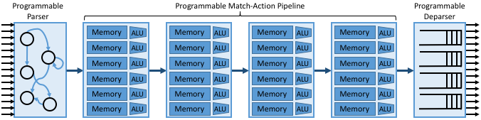
Figure 19. High-level overview of PISA’s multi-stage pipeline.

The individual Match-Action Units in Figure 19 deserve a closer look. The memory shown in the figure is typically built using a combination of SRAM and TCAM: it implements a table that stores bit patterns to be matched in the packets being processed. The relevance of the specific combination of memories is that TCAM is more expensive and power-hungry than SRAM, but it is able to support wildcard matches. Specifically, the “CAM” in TCAM stands for “Content Addressable Memory,” which means that the key you want to look up in a table can effectively be used as the address into the memory that implements the table. The “T” stands for “Ternary” which is a technical way to say the key you want to look up can have wildcards in it (e.g., key 10*1 matches both 1001 and 1011). From the software perspective, the main takeaway is that wildcard matches are more expensive than exact matches, and should be avoided when possible.

The ALU shown in the figure then implements the action paired with the corresponding pattern. Possible actions include modifying specific header fields (e.g., decrementing a TTL), pushing or popping tags (e.g., VLAN, MPLS), incrementing or clearing various counters internal to the switch (e.g., packets processed), and setting user/internal metadata (e.g. the VRF ID to be used in the routing table).

Directly programming the parser, match-action units, and deparser would be tedious, akin to writing microprocessor assembly code, so instead we express the desired behavior using a high-level language like P4, and depend on a compiler to generate the equivalent low-level program. We will get to the specifics of P4 in a later section, so for now we substitute an even more abstract representation of the desired forwarding pipeline: the graphical depiction included in Figure 20. (To be consistent with other examples, we call this program forward.p4.) This example program first matches L2 header fields, then matches either IPv4 or IPv6 header fields, and finally applies some ACL rules to the packets before allowing them through (e.g., think of the latter as firewall filter rules). This is an example of the OpenFlow pipeline shown in Figure 7 of Section 1.2.3.

In addition to translating the high-level representation of the pipeline onto the underlying PISA stages, the P4 compiler is also responsible for allocating the available PISA resources. In this case, there are four slots (rows) for the available Match-Action Units just as in Figure 19. Allocating slots in the available Match-Action units is the P4/PISA counterpart of register allocation for a conventional programming language running on a general-purpose microprocessor. In our example, we assume there are many more IPv4 Match-Action rules than IPv6 or ACL rules, so the compiler allocates entries in the available Match-Action Units accordingly.

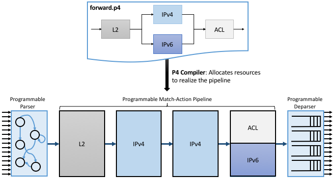
Figure 20. Depiction of the desired forwarding behavior (as specified by a pictorial representation of a P4 program) mapped onto PISA.

4.3 Abstracting the Pipeline

The next piece of the puzzle is to account for different switching chips implementing different physical pipelines. To do this we need an abstract (canonical) pipeline that is general enough to fairly represent the available hardware, plus a definition of how the abstract pipeline maps onto the physical pipeline. With such a logical model for the pipeline, we will be able to support pipeline-agnostic controllers, as illustrated in Figure 21.

Ideally, there will be just one logical pipeline, and the P4 compiler will be responsible for mapping that logical pipeline into various physical counterparts. Unfortunately, the marketplace has not yet converged on a single logical pipeline, but let’s put that complication aside for now. On the other side of the equation, there are currently on the order of ten target ASICs that this approach needs to account for. There are many more than ten switch vendors, but in practice, it is only those built for the high-end of the market that come into play.

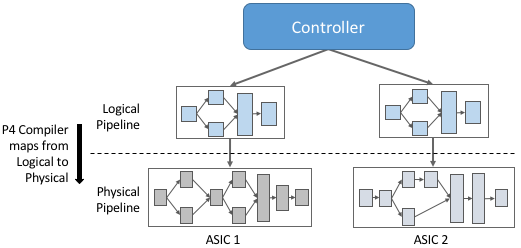
Figure 21. Defining a logical pipeline as a general approach to supporting a pipeline-agnostic control plane.

How do we specify the logical pipeline? This is also done with a P4 program, resulting in the situation shown in Figure 22. Notice that we are revisiting the two P4 programs introduced in Figure 15. The first program (forward.p4) defines the functionality we want from the available switching chip. This program is written by the developers who want to establish the behavior of the data plane. The second program (arch.p4) is essentially a header file: it represents a contract between the P4 program and the P4 compiler. Specifically, arch.p4 defines what P4-programmable blocks are available, the interface for each stage, and the capability for each stage. Who is responsible for writing such an architecture program? The P4 Consortium is one source of such a definition, but different switch vendors have created their own architecture specifications to closely describe the capabilities of their switching chips. This makes sense because there is a tension between having a single common architecture that enables executing the same P4 program on different ASICs from different vendors, and having an architecture that best represents the differentiating capabilities of any given ASIC.

The example shown in Figure 22 is called the Portable Switch Architecture (PSA). It is intended to provide P4 developers implementing forwarding programs like forward.p4 with an abstract target machine, analogous to a Java Virtual Machine. The goal is the same as for Java: to support a write-once-run-anywhere programming paradigm. (Note that Figure 22 includes the generic arch.p4 as the architecture model spec, but in practice the architecture model would be PSA specific, such as psa.p4.)

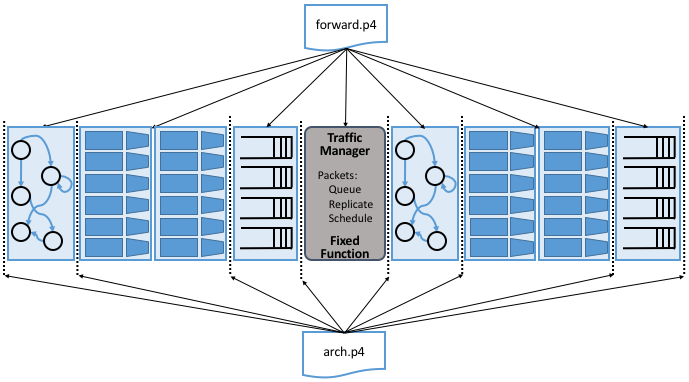
Figure 22. P4 architecture known as the Portable Switch Architecture (PSA). Includes the generic arch.p4 as the architecture model spec, but for PSA this would be replaced by psa.p4.

When compared to the simpler PISA model used in Figure 19 and 20, we see two major differences. First, the pipeline includes a new fixed-function stage: the Traffic Manager. This stage is responsible for queuing, replicating, and scheduling packets. This stage can be configured in well-defined ways (e.g., setting parameters such as queue size and scheduling policy), but cannot be re-programmed in a general-purpose way (e.g., to define a new scheduling algorithm). Second, the pipeline is divided into two halves: ingress processing (to the left of the Traffic Manager), and egress processing (to the right of the Traffic Manager).

What exactly does arch.p4 define? Essentially three things:

1. As implied by Figure 22, it defines the inter-block interface signatures in terms of input and output signals (think “function parameters and return type”). The goal of a P4 programmer to provide an implementation for each P4-programmable block that takes the provided input signals, such as the input port where a packet was received, and writes to the output signals to influence the behavior of the following blocks (e.g., the output queue/port where a packet has to be directed).

2. Type declarations for externs, which can be seen as additional fixed-function services that are exposed by the target and which can be invoked by a P4 programmer. Examples of such externs are checksum and hash computation units, packet or byte counters, ciphers to encrypt/decrypt the packet payload, and so on. The implementation of such externs is not specified in P4 by the architecture, but their interface is.

3. Extensions to core P4 language types, including alternative match types (e.g., range and lpm described in Section 4.4.3).

The P4 compiler (like all compilers) has a hardware-agnostic frontend that generates an Abstract Syntax Tree (AST) for the programs being compiled, and a hardware-specific backend that outputs an ASIC-specific executable. arch.p4 is simply a collection of type and interface definitions.

4.3.1 V1Model

The PSA shown in Figure 22 is still a work-in-progress. It represents an idealized architecture that sits between the P4 developer and the underlying hardware, but the architectural model that developers are coding to today is somewhat simpler. That model, called V1Model, is shown in Figure 23.1 It does not include a re-parsing step after the Traffic Manager. Instead it implicitly bridges all metadata from ingress to egress processing. Also, V1Model includes a checksum verification/update block, whereas PSA treats checksums as an extern, and supports incremental computations at any point during ingress/egress processing.

1

V1Model was originally introduced as the reference architecture for an earlier version of P4, known as P4_14, and was subsequently used to ease the porting of P4 programs from P4_14 to P4_16.

We will be using this simpler model throughout the rest of the book. As an aside, the most important factor in why V1Model is widely used and that is not the case for PSA, is that the switch vendors do not provide the compiler backend that maps from PSA onto their respective ASICs. Until that happens, PSA will remain a mostly “on paper” artifact.

Figure 23. V1Model used in practice to abstract away the details of different physical forwarding pipelines. Developers write P4 to this abstract architectural model.

When we say P4 developers “write to this model” we are being more descriptive than you might think. In practice, every P4 program starts with the following template, which literally has a code block for every programmable element in the abstract depiction shown in Figure 23.

#include <core.p4>
#include <v1model.p4>

/* Headers */
struct metadata { ... }
struct headers {
	ethernet_t	ethernet;
	ipv4_t		ipv4;
}

/* Parser */
parser MyParser(
	packet_in packet,
	out headers hdr,
	inout metadata meta,
	inout standard_metadata_t smeta) {
    ...
}

/* Checksum Verification */
control MyVerifyChecksum(
	in headers, hdr,
	inout metadata meta) {
    ...
}

/* Ingress Processing */
control MyIngress(
	inout headers hdr,
	inout metadata meta,
	inout standard_metadata_t smeta) {
    ...
}

/* Egress Processing */
control MyEgress(
	inout headers hdr,
	inout metadata meta,
	inout standard_metadata_t smeta) {
    ...
}

/* Checksum Update */
control MyComputeChecksum(
	inout headers, hdr,
	inout metadata meta) {
    ...
}

/* Deparser */
parser MyDeparser(
	inout headers hdr,
	inout metadata meta) {
    ...
}

/* Switch */
V1Switch(
    MyParser(),
    MyVerifyChecksum(),
    MyIngress(),
    MyEgress(),
    MyComputeChecksum(),
    MyDeparser()
) main;

That is, after including two definition files (core.p4, v1model.p4) and defining the packet headers that the pipeline is going to process, the programmer writes P4 code blocks for parsing, checksum verification, ingress processing, and so on. The final block (V1Switch) is the “main” function that specifies all the pieces are to be pulled together into a complete switch pipeline. As to the details corresponding to every “…” in the template, we will return to those in a later section. For now, the important point is that forward.p4 is a highly stylized program that gets its structure from the abstract model defined in v1model.p4.

4.3.2 TNA

As just noted, V1Model is one of many possible pipeline architectures. PSA is another, but it is also the case that different switch vendors have provided their own architecture definitions. There are different incentives for doing this. One is that vendors have their own version of the multi-ASIC problem as they continue to release new chips over time. Another is that it enables vendors to expose unique capabilities of their ASICs without being constrained by a standardization process. The Tofino Native Architecture (TNA), which is an architecture model defined by Barefoot for their family of programmable switching chips, is an example.

We aren’t going to describe TNA in detail here (information is available on GitHub for those that want a closer look), but having a second tangible example does help to illustrate all the degrees of freedom available in this space. In effect, the P4 language defines a general framework for writing programs (we’ll see the syntax in the next section), but it’s not until you supply a P4 architecture definition (generically we refer to this as arch.p4, but specific examples are v1model.p4, psa.p4, and tna.p4) that a developer is able to actually write and compile a forwarding program.

Further Reading

Open Tofino. 2021.

In contrast to v1model.p4 and psa.p4, which aspire to abstracting commonality across different switching chips, architectures like tna.p4 faithfully define the low-level capabilities of a given chip. Often, such capabilities are those that differentiate a chip like Tofino from the competition. When picking an architecture model for a new P4 program, it is important to ask questions like: Which of the available architectures are supported by the switches I intend to program? Does my program need access to chip-specific capabilities (e.g., a P4 extern to encrypt/decrypt packet payload) or can it rely solely on common/non-differentiating features (e.g., simple match-action tables or a P4 extern to count packets)?

As for that forwarding program (which we’ve been generically referring to as forward.p4), an interesting tangible example is a program that faithfully implements all the features that a conventional L2/L3 switch supports. Let’s call that program switch.p4.2 Strangely enough, that leaves us having re-created the legacy switch we could have bought from dozens of vendors, but there are two notable differences: (1) we can control that switch using an SDN controller via P4Runtime, and (2) we can easily modify that program should we discover we need a new feature.

2

Such a program was written by Barefoot for their chipset and uses tna.p4 as its architecture model, but it is not open source. A roughly equivalent open source variant, called fabric.p4, uses v1model.p4. It supports most L2/L3 features, customized for the SD-Fabric use case presented in Chapter 7.

Is the Complexity Worth It?

At this point you may be wondering if all the complexity being introduced is worth it, and we haven’t even gotten to the control plane yet! What we’ve covered so far is complex with or without SDN. That’s because we’re working at the SW/HW boundary, and the hardware is designed to forward packets at rates measured in Terabits-per-second. This complexity use to be hidden inside proprietary devices. One thing SDN has done is put pressure on the marketplace to open up that space so others can innovate.

But before anyone can innovate, the first step is to reproduce what we had running before, except now using open interfaces and programmable hardware. Even though this chapter uses forward.p4 as a hypothetical new data plane function someone might write, it’s really programs like switch.p4 (plus the Switch OS described in the next chapter) that establish parity with legacy networking gear. Once we have that in place, we are ready to do something new. But what?

It is not our goal to answer that question with any certainty. The VNF off-loading and INT examples introduced in Chapter 2 are a start. Software-defined 5G networks (Chapter 9) and closed-loop verification (Chapter 10) are potential killer-apps. But history teaches us that killer-apps are impossible to predict with any accuracy. On the other hand, history also includes many examples of how opening closed, fixed-function systems leads to qualitatively new capabilities.

To summarize, the overarching goal is to enable the development of control apps without regard to the specific details of the device forwarding pipeline. Introducing the P4 architecture model helps meet this goal, as it enables portability of the same forwarding pipeline (P4 program) across multiple targets (switching chips) that support the corresponding architecture model. However, it doesn’t totally solve the problem because the industry is still free to define multiple forwarding pipelines. But looking beyond the current state-of-affairs, having one or more programmable switches opens the door to programming the control app(s) and the forwarding pipeline in tandem. When everything is programmable, all the way down to the chip that forwards packets in the data plane, exposing that programmability to developers is the ultimate goal. If you have an innovative new function you want to inject into the network, you write both the control plane and data plane halves of that function, and turn the crank on the toolchain to load them into the SDN software stack! This is a significant step forward from a few years ago, where you might have been able to modify a routing protocol (because it was all in software) but you had no chance to change the forwarding pipeline because it was all in fixed-function hardware.

4.4 P4 Programs

Finally, we give a brief overview of the P4 language. The following is not a comprehensive reference manual for P4. Our more modest goal is to give a sense of what a P4 program looks like, thereby connecting all the dots introduced up to this point. We do this by example, that is, by walking through a P4 program that implements basic IP forwarding. This example is taken from a P4 Tutorial that you can find online and try for yourself.

Further Reading

P4 Tutorials. P4 Consortium, May 2019.

To help set some context, think of P4 as similar to the C programming language. P4 and C share a similar syntax, which makes sense because both are designed for low-level systems code. Unlike C, however, P4 does not include loops, pointers, or dynamic memory allocation. The lack of loops makes sense when you remember that we are specifying what happens in a single pipeline stage. In effect, P4 “unrolls” the loops we might otherwise need, implementing each iteration in one of a sequence of control blocks (i.e., stages). In the example program that follows, you can imagine plugging each code block into the template shown in the previous section.

4.4.1 Header Declarations and Metadata

First comes the protocol header declarations, which for our simple example includes the Ethernet and IP headers. This is also a place to define any program-specific metadata we want to associate with the packet being processed. The example leaves this structure empty, but v1model.p4 defines a standard metadata structure for the architecture as a whole. Although not shown in the following code block, this standard metadata structure includes such fields as ingress_port (port the packet arrived on), egress_port (port selected to send the packet out on), and drop (bit set to indicate the packet is to be dropped). These fields can be read or written by the functional blocks that make up the rest of the program.3

3

A quirk of the V1Model is that there are two egress port fields in the metadata structure. One (egress_port) is read-only and valid only in the egress processing stage. A second (egress_spec), is the field that gets written from the ingress processing stage to pick the output port. PSA and other architectures solve this problem by defining different metadata for the ingress and egress pipelines.

/***** P4_16 *****/
#include <core.p4>
#include <v1model.p4>

const bit<16> TYPE_IPV4 = 0x800;

/****************************************************
************* H E A D E R S  ************************
****************************************************/

typedef bit<9>  egressSpec_t;
typedef bit<48> macAddr_t;
typedef bit<32> ip4Addr_t;

header ethernet_t {
    macAddr_t dstAddr;
    macAddr_t srcAddr;
    bit<16>   etherType;
}

header ipv4_t {
    bit<4>    version;
    bit<4>    ihl;
    bit<8>    diffserv;
    bit<16>   totalLen;
    bit<16>   identification;
    bit<3>    flags;
    bit<13>   fragOffset;
    bit<8>    ttl;
    bit<8>    protocol;
    bit<16>   hdrChecksum;
    ip4Addr_t srcAddr;
    ip4Addr_t dstAddr;
}

struct metadata {
   /* empty */
}

struct headers {
    ethernet_t   ethernet;
    ipv4_t       ipv4;
}

4.4.2 Parser

The next block implements the parser. The underlying programming model for the parser is a state transition diagram, including the built-in start, accept, and reject states. The programmer adds other states (parse_ethernet and parse_ipv4 in our example), plus the state transition logic. For example, the following parser always transitions from the start state to the parse_ethernet state, and if it finds the TYPE_IPV4 (see the constant definition in the previous code block) in the etherType field of the Ethernet header, next transitions to the parse_ipv4 state. As a side-effect of traversing each state, the corresponding header is extracted from the packet. The values in these in-memory structures are then available to the other routines, as we will see below.

/****************************************************
************* P A R S E R  **************************
****************************************************/

parser MyParser(
	packet_in packet,
	out headers hdr,
	inout metadata meta,
	inout standard_metadata_t standard_metadata) {

    state start {
        transition parse_ethernet;
    }

    state parse_ethernet {
        packet.extract(hdr.ethernet);
        transition select(hdr.ethernet.etherType) {
            TYPE_IPV4: parse_ipv4;
            default: accept;
        }
    }

    state parse_ipv4 {
        packet.extract(hdr.ipv4);
        transition accept;
    }
}

As is the case with all the code blocks in this section, the function signature for the parser is defined by the architecture model, in this case, v1model.p4. We do not comment further on the specific parameters, except to make the general observation that P4 is architecture-agnostic. The program you write depends heavily on the architecture model you include.

4.4.3 Ingress Processing

Ingress processing has two parts. The first is checksum verification.4 This is minimal in our example; it simply applies the default. The interesting new feature this example introduces is the control construct, which is effectively P4’s version of a procedure call. While it is possible for a programmer to also define “subroutines” as their sense of modularity dictates, at the top level these control blocks match up one-for-one with the pipeline stages defined by the logical pipeline model.

4

This is particular to V1Model. PSA doesn’t have an explicit checksum verification or computation stage of ingress or egress respectively.

/****************************************************
***  C H E C K S U M    V E R I F I C A T I O N   ***
****************************************************/

control MyVerifyChecksum(
	inout headers hdr,
	inout metadata meta) {   
    apply {  }
}

We now get to the heart of the forwarding algorithm, which is implemented in the ingress segment of the Match-Action pipeline. What we find are two actions being defined: drop() and ipv4_foward(). The second of these two is the interesting one. It takes a dstAddr and an egress port as arguments, assigns the port to the corresponding field in the standard metadata structure, sets the srcAddr/dstAddr fields in the packet’s ethernet header, and decrements the ttl field of the IP header. After executing this action, the headers and metadata associated with this packet contain enough information to properly carry out the forwarding decision.

But how does that decision get made? This is the purpose of the table construct. The table definition includes a key to be looked up, a possible set of actions (ipv4_forward, drop, NoAction), the size of the table (1024 entries), and the default action to take whenever there is no match in the table (drop). The key specification includes both the header field to be looked up (the dstAddr field of the IPv4 header), and the type of match we want (lpm implies Longest Prefix Match). Other possible match types include exact and ternary, the latter of which effectively applies a mask to select which bits in the key to include in the comparison. lpm, exact and ternary are part of the core P4 language types, where their definitions can be found in core.p4. P4 architectures can expose additional match types. For example, PSA also defines range and selector matches.

The final step of the ingress routine is to “apply” the table we just defined. This is done only if the parser (or previous pipeline stage) marked the IP header as valid.

/****************************************************
******  I N G R E S S   P R O C E S S I N G   *******
****************************************************/

control MyIngress(
	inout headers hdr,
	inout metadata meta,
	inout standard_metadata_t standard_metadata) {			

    action drop() {
        mark_to_drop(standard_metadata);
    }
    
    action ipv4_forward(macAddr_t dstAddr,
			egressSpec_t port) {
	standard_metadata.egress_spec = port;
        hdr.ethernet.srcAddr = hdr.ethernet.dstAddr;
        hdr.ethernet.dstAddr = dstAddr;
        hdr.ipv4.ttl = hdr.ipv4.ttl - 1;
    }
    
    table ipv4_lpm {
        key = {
            hdr.ipv4.dstAddr: lpm;
        }
        actions = {
            ipv4_forward;
            drop;
            NoAction;
        }
        size = 1024;
       default_action = drop();
    }
   
    apply {
        if (hdr.ipv4.isValid()) {
            ipv4_lpm.apply();
        }
   }
}

4.4.4 Egress Processing

Egress processing is a no-op in our simple example, but in general it is an opportunity to perform actions based on the egress port, which might not be known during ingress processing (e.g., it might depend on the traffic manager). For example, replicating a packet to multiple egress ports for multicast can be done by setting the corresponding intrinsic metadata in the ingress processing, where the meaning of such metadata is defined by the architecture. The egress processing will see as many copies of the same packet as those generated by the traffic manager. As a second example, if one switch port is expected to send VLAN-tagged packets, the header must be extended with the VLAN id. A simple way of dealing with such a scenario is by creating a table that matches on the egress_port of the metadata. Other examples include doing ingress port pruning for multicast/broadcast packets and adding a special “CPU header” for intercepted packets passed up to the control plane.

/****************************************************
*******  E G R E S S   P R O C E S S I N G   ********
****************************************************/

control MyEgress(
	inout headers hdr,
	inout metadata meta,
	inout standard_metadata_t standard_metadata) {
   
    apply {  }
}

/****************************************************
***   C H E C K S U M    C O M P U T A T I O N   ****
****************************************************/

control MyComputeChecksum(
	inout headers  hdr,
	inout metadata meta) {
   
     apply {
	update_checksum(
	    hdr.ipv4.isValid(),
              { hdr.ipv4.version,
	        hdr.ipv4.ihl,
                hdr.ipv4.diffserv,
                hdr.ipv4.totalLen,
                hdr.ipv4.identification,
                hdr.ipv4.flags,
                hdr.ipv4.fragOffset,
                hdr.ipv4.ttl,
                hdr.ipv4.protocol,
                hdr.ipv4.srcAddr,
                hdr.ipv4.dstAddr },
            hdr.ipv4.hdrChecksum,
            HashAlgorithm.csum16);
    }
}

4.4.5 Deparser

The deparser is typically straightforward. Having potentially changed various header fields during packet processing, we now have an opportunity to emit the updated header fields. If you change a header in one of your pipeline stages, you need to remember to emit it. Only headers that are marketed as valid will be re-serialized into that packet. There is no need to say anything about the rest of the packet (i.e., the payload), since by default, all the bytes beyond where we stopped parsing are included in the outgoing message. The details of how packets are emitted are specified by the architecture. For example, TNA supports truncating the payload based on the setting of a special metadata value consumed by the deparser.

/****************************************************
*************  D E P A R S E R  *********************
****************************************************/

control MyDeparser(
	packet_out packet,
	in headers hdr) {
		
    apply {
        packet.emit(hdr.ethernet);
        packet.emit(hdr.ipv4);
    }
}

4.4.6 Switch Definition

Finally, the P4 program must define the behavior of the switch as a whole, which is given by the V1Switch package shown below. This set of elements in this package is defined by v1model.p4, and consists of references to all the other routines defined above.

/****************************************************
*************  S W I T C H  *************************
****************************************************/

V1Switch(
    MyParser(),
    MyVerifyChecksum(),
    MyIngress(),
    MyEgress(),
    MyComputeChecksum(),
    MyDeparser()
) main;

Keep in mind this example is minimal, but it does serve to illustrate the essential ideas in a P4 program. What’s hidden by this example is the interface used by the control plane to inject data into the routing table; table ipv4_lpm defines the table, but does not populate it with values. We resolve the mystery of how the control plane puts values into the table when we discuss P4Runtime in Chapter 5.

4.5 Fixed-Function Pipelines

We now return to fixed-function forwarding pipelines, with the goal of placing them in the larger ecosystem. Keeping in mind that fixed-function switching chips still dominate the market, we do not mean to understate their value or the role they will undoubtedly continue to play.5 But they do remove one degree-of-freedom—the ability to reprogram the data plane—which helps to highlight the relationship between all the moving parts introduced in this chapter.

5

The distinction between fixed-function and programmable pipelines is not as black-and-white as this discussion implies, since fixed-function pipelines can also be configured. But parameterizing a switching chip and programming a switching chip are qualitatively different, with only the latter able to accommodate new functionality.

4.5.1 OF-DPA

We start with a concrete example: The OpenFlow—Data Plane Abstraction (OF-DPA) hardware abstraction layer that Broadcom provides for their switching chips. OF-DPA defines an API that can be used to install flow rules into the underlying Broadcom ASIC. Technically, an OpenFlow agent sits on top of OF-DPA (it implements the over-the-wire aspects of the OpenFlow protocol) and the Broadcom SDK sits below OF-DPA (it implements the proprietary interface that knows about the low-level chip details), but OF-DPA is the layer that provides an abstract representation of the Tomahawk ASIC’s fixed forwarding pipeline. Figure 24 shows the resulting software stack, where OF-Agent and OF-DPA are open source (the OF-Agent corresponds to a software module called Indigo, originally written by Big Switch), whereas the Broadcom SDK is proprietary. Figure 25 then depicts what the OF-DPA pipeline looks like.

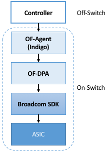
Figure 24. Software stack for Tomahawk fixed-function forwarding pipeline.

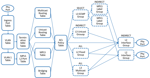
Figure 25. Logical fixed-function pipeline defined by OF-DPA.

We do not delve into the details of Figure 25, but the reader will recognize tables for several well-known protocols. For our purposes, what is instructive is to see how OF-DPA maps onto its programmable pipeline counterparts. In the programmable case, it’s not until you add a program like switch.p4 that you get something roughly equivalent to OF-DPA. That is, v1model.p4 defines the available stages (control blocks). But it’s not until you add switch.p4 that you have the functionality that runs in those stages.

With this relationship in mind, we might want to incorporate both programmable and fixed-function switches in a single network and running a common SDN software stack. This can be accomplished by hiding both types of chips behind the v1model.p4 (or similar) architecture model, and letting the P4 compiler output the backend code understood by their respective SDKs. Obviously this scenario doesn’t work for an arbitrary P4 program that wants to do something that the Tomahawk chip doesn’t support, but it will work for standard L2/L3 switch behavior.

4.5.2 SAI

Just as we saw both vendor-defined and community-defined architecture models (TNA and V1Model, respectively), there are also vendor-defined and community-defined logical fixed-function pipelines. OF-DPA is the former, and the Switch Abstraction Interface (SAI) is an example of the latter. Because SAI has to work across a range of switches—and forwarding pipelines—it necessarily focuses on the subset of functionality all vendors can agree on, the least common denominator, so to speak.

SAI includes both a configuration interface and a control interface, where it’s the latter that is most relevant to this section because it abstracts the forwarding pipeline. On the other hand, there is little value in looking at yet another forwarding pipeline, so we refer the interested reader to the SAI specification for more details.

Further Reading

SAI Pipeline Behavioral Model. Open Compute Project.

We revisit the configuration API in the next chapter.

4.6 Comparison

This discussion about logical pipelines and their relationship to P4 programs is subtle, and worth restating. On the one hand, there is obvious value in having an abstract representation of a physical pipeline, as introduced as a general concept in Figure 21. When used in this way, a logical pipeline is an example of the tried-and-true idea of introducing a hardware abstraction layer. In our case, it helps with control plane portability. OF-DPA is a specific example of a hardware abstraction layer for Broadcom’s fixed-function switching chips.

On the other hand, P4 provides a programming model, with architectures like v1model.p4 and tna.p4 adding detail to P4’s general language constructs (e.g., control, table, parser). These architecture models are, in effect, a language-based abstraction of a generic forwarding device, which can be fully-resolved into a logical pipeline by adding a particular P4 program like switch.p4. P4 architecture models don’t define pipelines of match-action tables, but they instead define the building blocks (including signatures) that can be used by a P4 developer to define a pipeline, whether logical or physical. In a sense, then, P4 architectures are equivalent to a traditional switch SDK, as illustrated by the five side-by-side examples in Figure 26.

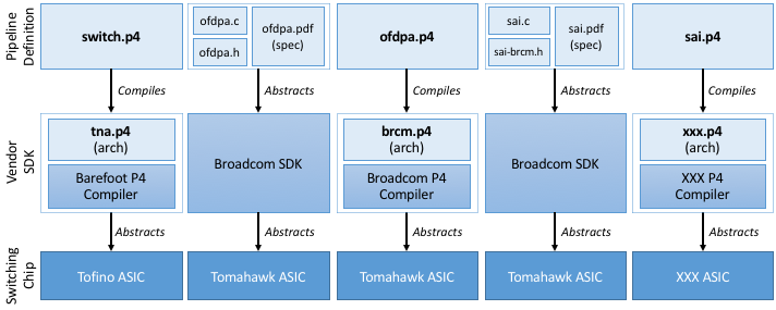
Figure 26. Five example Pipeline/SDK/ASIC stacks. The two leftmost stacks, plus the fourth stack, exist today; the middle stack is hypothetical; and the rightmost stack is a work-in-progress.

Each example in Figure 26 consists of three layers: a switching chip ASIC, a vendor-specific SDK for programming the ASIC, and a definition of the forwarding pipeline. By providing a programmatic interface, the SDKs in the middle layer effectively abstract the underlying hardware. They are either conventional (e.g., the Broadcom SDK shown in the second and fourth examples) or, as just pointed out, logically correspond to a P4 architecture model paired with an ASIC-specific P4 compiler. The topmost layer in all five examples defines a logical pipeline that can subsequently be controlled using a control interface like OpenFlow or P4Runtime (not shown). The five examples differ based on whether the pipeline is defined by a P4 program or through some other means (e.g., the OF-DPA specification).

Note that only those configurations with a P4-defined logical pipeline at the top of the stack (i.e., first, third, fifth examples) can be controlled using P4Runtime. This is for the pragmatic reason that the P4Runtime interface is auto-generated from this P4 program using the tooling described in the next Chapter.

The two leftmost examples exist today, and represent the canonical layers for programmable and fixed-function ASICs, respectively. The middle example is purely hypothetical, but it illustrates that it is possible to define a P4-based stack even for a fixed-function pipeline (and, by implication, control it using P4Runtime). The fourth example also exists today, and is how Broadcom ASICs conform to the SAI-defined logical pipeline. Finally, the rightmost example projects into the future, when SAI is extended to support P4 programmability and runs on multiple ASICs.